8. MTfit.algorithms: Search Algorithms
These algorithms and their effects are explored in Pugh (2015), which expands in further detail on the topics covered here.
8.1. Table Of Contents:
8.2. Algorithms
This module contains the sampling approaches used. Two main approaches are used:
- Random Monte Carlo sampling
- Markov chain Monte Carlo sampling
However, there are also two variants of the Markov chain Monte Carlo (McMC) method:
- Metropolis-Hastings
- Trans-Dimensional Metropolis-Hastings (Reversible Jump)
8.3. Random Monte Carlo sampling
The simplest approach is that of random sampling over the moment tensor or double-couple space. Stochastic Monte Carlo sampling introduces no biases and provides an estimate for the true PDF, but requires a sufficient density of sampling to reduce the uncertainties in the estimate. The sampled PDF approaches the true distribution in the limit of infnite samples. However, this approach is limited both by time and memory. Some benefits can be gained by only keeping the samples with non-zero probability.
The assumed prior distribution is a uniform distribution on the unit 6-sphere in moment tensor space. This is equivalent to unit normalisation of the moment tensor six vector:
This sampling is explored further in Pugh et al, 2015t.
8.4. Markov chain Monte Carlo sampling
An alternative approach is to use Markov chain Monte Carlo (McMC) sampling. This constructs a Markov chain (Norris, 1998) of which the equilibrium distribution is a good sample of the target probability distribution.
A Markov chain is a memoryless stochastic process of transitioning between states. The probability of the next value depends only on the current value, rather than all the previous values, which is known as the Markov property (Markov, 1954):
A suitable McMC method should converge on the target distribution rapidly. As an approach it is more complex than the Monte Carlo random sampling approach described above, and by taking samples close to other non-zero samples, there is moreintelligence to the sampling than in the random Monte Carlo sampling approach.
A Metropolis-Hastings approach is used here (Metropolis, 1953 and Hastings, 1970). The Metropolis-Hastings approach is a common method for McMC sampling and satisfies the detailed balance condition (Robert and Casella, 2004, eq. 6.22), which means that the probability density of the chain is stationary. New samples are drawn from a probability density \(\mathrm{q}\left(\mathbf{x'}|\mathbf{x}_\mathrm{t}\right)\) to evaluate the target probability density \(\mathrm{p}\left(\mathbf x|\mathbf d\right)\).
The Metropolis-Hastings algorithm begins with a random starting point and then iterates until this initial state is forgotten (Algorithm). Each iteration evaluates whether a new proposed state is accepted or not. If \(\mathrm{q}\left(\mathbf{x'}|\mathbf{x}_\mathrm{t}\right)\) is symmetric, then the ratio \(\frac{\mathrm{q}\left(\mathbf{x}_\mathrm{t}|\mathbf{x'}\right)}{\mathrm{q}\left(\mathbf{x'}|\mathbf{x}_\mathrm{t}\right)}=1\). The acceptance, alpha, is given by
which can be expanded using Bayes' Theorem to give the acceptance in terms of the likelihood \(\mathrm{p}\left(\mathbf d|\mathbf x\right)\) and prior \(\mathrm{p}\left(\mathbf x\right)\),
The acceptance is the probability that the new sample in the chain, \(\mathbf{x}_\mathrm{t+1}\) is the new sample, \(\mathbf{x'}\), otherwise the original value, \(\mathbf{x}_\mathrm{t}\) , is added to the chain again,
The algorithm used in MTfit is:
| Metropolis-Hastings Markov chain Monte Carlo Sampling Algorithm | ||
|---|---|---|
| 1 | Determine initial value for \(\mathbf{x}_0\) with non-zero likelihood | |
| 2 | Draw new sample \(\mathbf{x'}\) from transition PDF \(\mathrm{q}\left(\mathbf{x'}|\mathbf{x}_\mathrm{t}\right)\) | |
| 3 | Evaluate likelihood for sample \(\mathbf{x'}\) | |
| 4 | Calculate acceptance, \(\alpha\), for \(\mathbf{x'}\). | |
| 5 | Determine sample \(\mathbf{x}_\mathrm{t+1}\). | |
| 6 | If in learning period: | |
| If sufficient samples (> 100) have been obtained, update transition PDF parameters to target ideal acceptance rate. | ||
| Return to 2 until end of learning period and discard learning samples. | ||
| Otherwise return to 2 until sufficient samples are drawn. | ||
The source parameterisation is from Tape and Tape (2012), and the algorithm uses an iterative parameterisation for the learning parameters during a learning period, then generates a Markov chain from the pdf.
8.4.1. Reversible Jump Markov chain Monte Carlo Sampling
The Metropolis-Hastings approach does not account for variable dimension models. Green (1995) introduced a new type of move, a jump, extending the approach to variable dimension problems. The jump introduces a dimension-balancing vector, so it can be evaluated like the normal Metropolis-Hastings shift.
Green (1995) showed that the acceptance for a pair of models \(M_\mathrm{t}\) and \(M'\) is given by:
where \(\mathrm{q}\left(\mathbf{x'}|\mathbf{x}_\mathrm{t}\right)\) is the probability of making the transition from parameters \(\mathbf{x}_\mathrm{t}\) from model \(M_\mathrm{t}\) to parameters \(\mathbf{x'}\) from model \(M'\), and \(\mathrm{p}\left(M_\mathrm{t}\right)\) is the prior for the model \(M_\mathrm{t}\).
If the models \(M_\mathrm{t}\) and \(M'\) are the same, the reversible jump acceptance is the same as the Metropolis-Hastings acceptance, because the model priors are the same. The importance of the reversible jump approach is that it allows a transformation between different models, and even different dimensions.
The dimension balancing vector requires a bijection between the parameters of the two models, so that the transformation is not singular and a reverse jump can occur. In the case where \(\dim\left(M'\right)>\dim\left(M_\mathrm{t}\right)\), a vector \(\mathbf u\) of length \(\dim\left(M'\right)-\dim\left(M_\mathrm{t}\right)\) needs to be introduced to balance the number of parameters in \(\mathbf{x'}\). The values of \(\mathbf u\) have probability density \(\mathrm{q}\left(\mathbf u\right)\) and some bijection that maps \(\mathbf{x}_\mathrm{t},\mathbf u\rightarrow\mathbf{x'}\), \(\mathbf{x'}=\mathrm{h}\left(\mathbf{x}_\mathrm{t},\mathbf u\right)\).
If the jump has a probability \(\mathrm{j}\left(\mathbf x\right)\) of occurring for a sample \(\mathbf x\), the transition probability depends on the jump parameters, \(\mathbf u\) and the transition ratio is given by:
with the Jacobian matrix, \(\mathbf J=\frac{\partial\mathrm{h}\left(\mathbf{x}_\mathrm{t},\mathbf u\right)}{\partial\left(\mathbf{x}_\mathrm{t},\mathbf u\right)}\).
The general form of the jump acceptance involves a prior on the models, along with a prior on the parameters. The acceptance for this case is:
If the jump is from higher dimensions to lower, the bijection describing the transformation has an inverse that describes the transformation \(\mathbf{x'}\rightarrow\mathbf{x}_\mathrm{t},\mathbf u\), and the acceptance is given by:
A simple example used in the literature (see Green, 1995; Brooks et al., 2003) is a mapping from a one dimensional model with parameter \(\theta\) to a two dimensional model with parameters \(\theta_{1},\theta_{2}\). A possible bijection is given by:
with the reverse bijection given by:
8.4.1.1. Reversible Jump McMC in Source Inversion
The reversible jump McMC approach allows switching between different source models, such as the double-couple model and the higher dimensional model of the full moment tensor, and can be extended to other source models.
The full moment tensor model is nested around the double-couple point, leading to a simple description of the jumps by keeping the common parameters constant. The Tape parameterisation (Tape and Tape, 2012) allows for easy movement both in the source space and between models. The moment tensor model has five parameters:
- strike \(\left(\kappa\right)\)
- dip cosine \(\left(h\right)\)
- slip \(\left(\sigma\right)\)
- eigenvalue co-latitude \(\left(\delta\right)\)
- eigenvalue longitude \(\left(\gamma\right)\)
while the double-couple model has only the three orientation parameters: \(\kappa\), \(h\), and \(\sigma\). Consequently, the orientation parameters are left unchanged between the two models, and the dimension balancing vector for the jump has two elements, which can be mapped to \(\gamma\) and \(\delta\):
The algorithm used is:
| Reversible Jump Markov chain Monte Carlo sampling Algorithm | ||
|---|---|---|
| 1 | Determine initial value for \(\mathbf{x}_0\) with non-zero likelihood | |
| 2 | Determine which move type to carry out: | |
| Carry out jump with probability \(p_\mathrm{jump}\): Draw new sample \(\mathbf{x'}=\left(\mathbf{x},\mathbf{u}\right)\) with dimension balancing vector \(\mathbf{u}\) drawn from \(\mathrm{q}\left(u1, u2\right)\). | ||
| Carry out shift with probability \(1-p_\mathrm{jump}\): Draw new sample \(\mathbf{x'}\) from transition PDF \(\mathrm{q}\left(\mathbf{x'}|\mathbf{x}_\mathrm{t}\right)\). | ||
| 3 | Evaluate likelihood for sample \(\mathbf{x'}\) | |
| 4 | Calculate acceptance, \(\alpha\), for \(\mathbf{x'}\). | |
| 5 | Determine sample \(\mathbf{x}_\mathrm{t+1}\). | |
| 6 | If in learning period: | |
| If sufficient samples (> 100) have been obtained, update transition PDF parameters to target ideal acceptance rate. | ||
| Return to 2 until end of learning period and discard learning samples. | ||
| Otherwise return to 2 until sufficient samples are drawn. | ||
8.5. Relative Amplitude
Inverting for multiple events increases the dimensions of the source space for each event. This leads to a much reduced probability of obtaining a non-zero likelihood sample, because sampling from the n-event distribution leads to multiplying the probabilities of drawing a non-zero samples, resulting in sparser sampling of the joint source PDF.
The elapsed time for the random sampling is longer per sample than the individual sampling, and longer than the combined sampling for both events due to evaluating the relative amplitude PDF. Moreover, increasing the number of samples 10-fold raises the required time by a factor of 10, requiring some method of reducing the running time for the inversion, since, given current processor speeds, \(10^{15}\) samples would take many years to calculate on a single core. As a result, more intelligent search algorithms are required for the full moment tensor case.
Markov chain approaches are less dependent on the model dimensionality. To account for the fact that the uncertainties in each parameter can differ between the events, the Markov chain shape parameters can be scaled based on the relative non-zero percentages of the events when they are initialised. The initialisation approaches also need to be adjusted to account for the reduced non-zero sample probability, such as by initialising the Markov chain independently for each event. The trans-dimensional McMC algorithm allows model jumping independently for each event.
Tuning the Markov chain acceptance rate is difficult, as it is extremely sensitive to small changes in the proposal distribution widths, and with the higher dimensionality it may be necessary to lower the targeted acceptance rate to improve sampling. Consequently, care needs to be taken when tuning the parameters to effectively implement the approaches for relative amplitude data.
8.6. Running Time
Comparing different sample sizes shows that the McMC approaches require far fewer samples than random sampling. However, the random sampling algorithm is quick to calculate the likelihood for a large number of samples, unlike the McMC approach, because of the extra computations in calculating the acceptance and obtaining new samples. Some optimisations have been included in the McMC algorithms, including calculating the probability for multiple new samples at once, with sufficient samples that there is a high probability of containing an accepted sample. This is more efficient than repeatedly updating the algorithm.
Despite these optimisations, the McMC approach is still much slower to reach comparable sample sizes, and is slower than would be expected just given the targeted acceptance rate, because of the additional computational overheads:
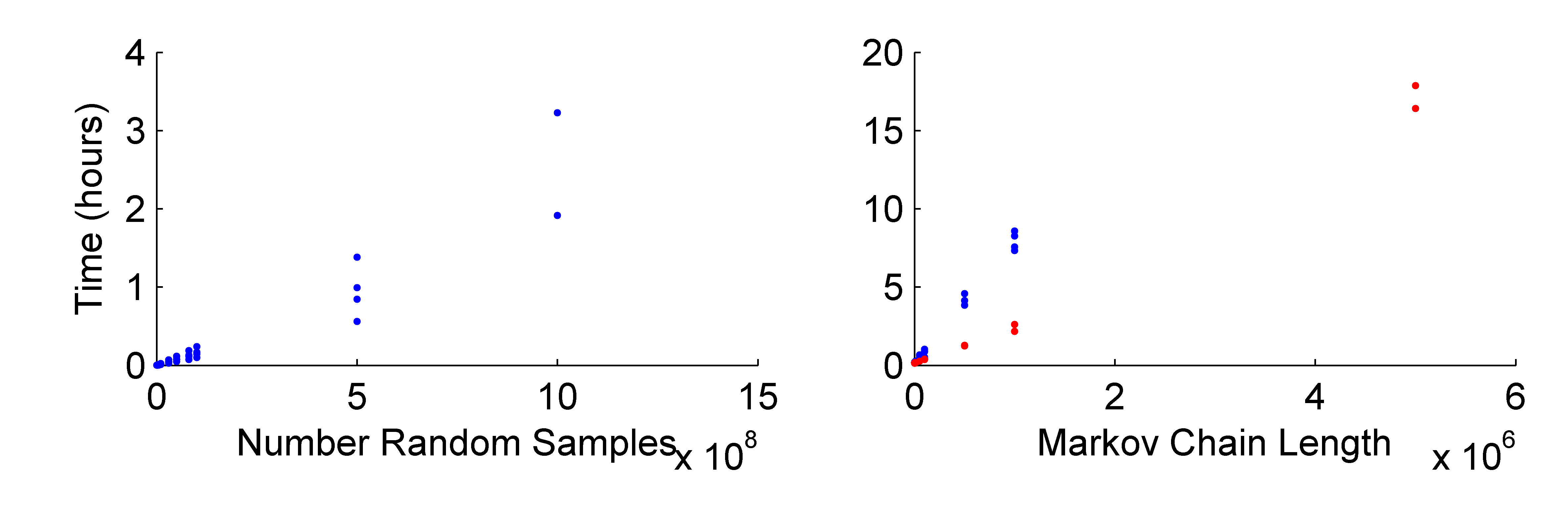
Elapsed Time for different sample sizes of the random sampling algorithm and for McMC algorithms with different number of unique samples.
Including location uncertainty and model uncertainty in the forward model causes a rapid reduction of the available samples for a given amount of RAM and increases the number of times the forward model must be evaluated, lengthening the time for sufficient sampling.
The location uncertainty has less of an effect on the McMC algorithms, since the number of samples being tested at any given iteration are small. Consequently, as the random sampling approach becomes slower, the fewer samples required to construct the Markov chain starts to produce good samples of the source PDF at comparable times. However, there is an initial offset in the elapsed time for the Markov chain Monte Carlo approaches due to the burn in and initialisation of the algorithm:
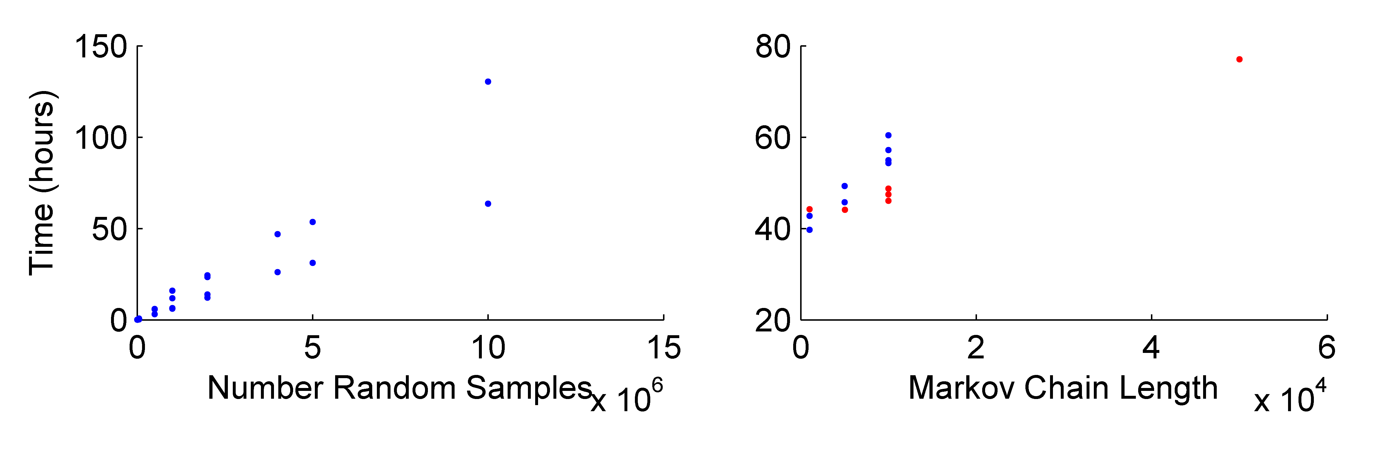
Elapsed Time for different sample sizes of the random sampling algorithm and for McMC algorithms with different number of unique samples. The velocity model and location uncertainty in the source was included with a one degree binning reducing the number of location samples from 50,000 to 5, 463.
The relative amplitude algorithms require an exponential increase in the number of samples as the number of events being sampled increases. However, the McMC approaches are more intelligent and do not require the same increase in sample size, but these algorithms can prove difficult to estimate the appropriate sampling parameters for the proposal distribution:
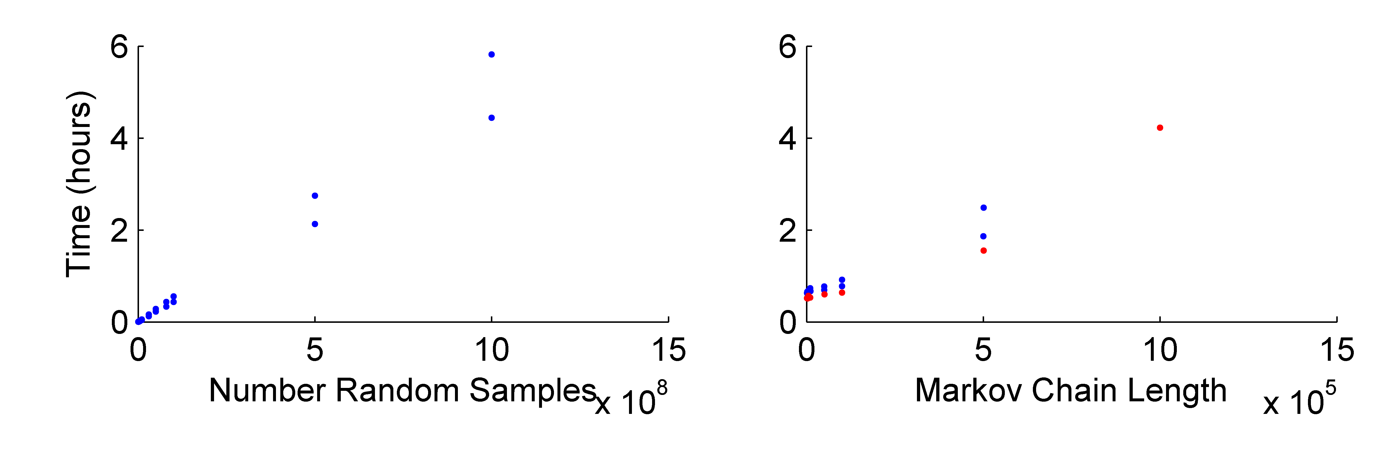
Elapsed Time for different sample sizes of the random sampling algorithm and for McMC algorithms with different number of unique samples for a two event joint PDF with relative P-amplitudes.
8.7. Summary
There are several different approaches to sampling for the forward model. The Monte Carlo random sampling is quick, although it requires a large number of samples to produce good samplings of the PDF. The McMC approaches produce good sampling of the source for far fewer samples, but the evaluation time can be long due to the overhead of calculating the acceptance and generating new samples. Furthermore, these approaches rely on achieving the desired acceptance rate to sufficiently sample the PDF given the chain length. Including location uncertainty increases the random sampling time drastically, and has less of an effect on the McMC approaches.
The solutions for the different algorithms and different source types are consistent, but the McMC approach can be poor at sampling multi-modal distributions if the acceptance rate is too high.
The two different approaches for estimating the probability of the double-couple source type model being correct are consistent, apart from cases where the PDF is dominated by a few very high probability samples. For these solutions, the number of random samples needs to be increased sufficiently to estimate the probability well. The McMC approach cannot easily be used to estimate the double-couple model probabilities, unlike both the random sampling and trans-dimensional approaches.
Extending these models to relative source inversion leads to a drastically increased number of samples required for the Monte Carlo random sampling approach that it becomes infeasible with current computation approaches. However, the McMC approaches can surmount this problem due to the improved sampling approach, but care must be taken when initialising the algorithm to make sure that sufficient samples are discarded that any initial bias has been removed, as well as targeting an acceptance rate that does not require extremely large chain lengths to successfully explore the full space.
The required number of samples depends on each event, and the constraint on the source that is given by the data. Usually including more data-types can sharpen the PDF, requiring more samples to get a satisfactory sampling of the event.