4. Tutorial: Using MTfit
MTfit is a bayesian approach to moment tensor inversion, allowing rigorous inclusion of uncertainties. This section shows a simple series of examples for running MTfit.
The example data is included in examples/example_data.py and are purely data that are used as an example, rather than a necessarily good solution.
These examples show some of the common usage of MTfit. However, the reasons behind the choice of approach have not always been well explained. The next page (Real Data Examples) includes real and synthetic data used in the Pugh et al. 2016a paper as an example of the results that can be obtained using MTfit, along with some explanation of the parameter choices made.
The tutorials described here are:
4.1. Creating a Data Dictionary
The input data dictionary (see Input Data) can either be pickled or not pickled. The structure is simple:
>>> import numpy as np
>>> data = {'PPolarity': {'Measured': np.matrix([[-1], [-1], [1], [1]]),
                          'Error': np.matrix([[0.01], [0.02], [0.4], [0.1]]),
                          'Stations':{'Name': ['Station1', 'Station2', 'Station3',
                                               'Station4'],
                                      'Azimuth': np.matrix([[248.0], [122.3],
                                                            [182.3], [35.2]]),
                                      'TakeOffAngle': np.matrix([[24.5], [22.8],
                                                                 [74.5], [54.3]])}},
          'UID': 'Event1'}
This has created a data dictionary for Event1 with P Polarity observations at 4 stations:
>>> print data
{'PPolarity': {'Stations': {'TakeOffAngle': matrix([[ 24.5],
        [ 22.8],
        [ 74.5],
        [ 54.3]]),
    'Name': ['Station1', 'Station2', 'Station3', 'Station4'],
    'Azimuth': matrix([[ 248. ],
        [ 122.3],
        [ 182.3],
        [  35.2]])},
    'Measured': matrix([[-1],
        [-1],
        [ 1],
        [ 1]]),
    'Error': matrix([[ 0.01],
        [ 0.02],
        [ 0.4 ],
        [ 0.1 ]])},
'UID': 'Event1'}
If there were more observations such as P/SH Amplitude Ratios, the data dictionary above would need to be updated:
>>> data['P/SHAmplitudeRatio'] = {'Measured': np.matrix([[1242, 1113], [742, 2341],
                                                         [421, 112], [120, 87]]),
                     'Error': np.matrix([[102, 743], [66, 45], [342, 98], [14, 11]]),
                     'Stations': {'Name': ['Station5', 'Station6',
                                    'Station7', 'Station8'],
                                 'Azimuth': np.matrix([[163.0], [345.3],
                                                       [25.3], [99.2]]),
                                 'TakeOffAngle': np.matrix([[51.5], [76.8],
                                                            [22.5], [11.3]]),
                                }
                     }
This has added P/SH Amplitude Ratio observations for 4 more stations to the data dictionary:
>>> print data
{'PPolarity': {'Stations': {'TakeOffAngle': matrix([[ 24.5],
        [ 22.8],
        [ 74.5],
        [ 54.3]]),
    'Name': ['Station1', 'Station2', 'Station3', 'Station4'],
    'Azimuth': matrix([[ 248. ],
        [ 122.3],
        [ 182.3],
        [  35.2]])},
    'Measured': matrix([[-1],
        [-1],
        [ 1],
        [ 1]]),
    'Error': matrix([[ 0.01],
        [ 0.02],
        [ 0.4 ],
        [ 0.1 ]])},
'P/SHAmplitudeRatio': {'Stations': {'TakeOffAngle': matrix([[ 51.5],
        [ 76.8],
        [ 22.5],
        [ 11.3]]),
    'Name': ['Station5', 'Station6', 'Station7', 'Station8'],
    'Azimuth': matrix([[ 163. ],
        [ 345.3],
        [  25.3],
        [  99.2]])},
    'Measured': matrix([[1242, 1113],
        [ 742, 2341],
        [ 421,  112],
        [ 120,   87]]),
    'Error': matrix([[102, 743],
        [ 66,  45],
        [342,  98],
        [ 14,  11]])},
'UID': 'Event1'}
The amplitude ratio Measured and Error numpy matrices have the observations of the ratio numerator and denominator at each station, i.e. in this case, Station5 has P Amplitude is 1242 and SH Amplitude is 1113, along with P error 102 and SH error 743. The split into numerator and denominator is required because the appropriate PDF is the ratio PDF (see Amplitude Ratio PDF).
This dictionary can either be provided as a construction argument for the Inversion object:
>>> import MTfit
>>> inversion_object = MTfit.Inversion(data)
>>> inversion_object.forward()
Or read in from the command line:
>>> import cPickle
>>> cPickle.dump(data, open('Event1.inv', 'wb'))
This has created a pickled dictionary called Event1.inv in the current directory. To perform the inversion, open a shell in the same directory:
$ MTfit -d Event1.inv
This will create an output file Event1MT.mat which contains the MATLAB output data (see Output).
The creation of the dictionary can easily be automated from different data types by writing a simple parser for the format.
4.2. P Polarity Inversion
Using the above tutorial, it is simple to carry out a P polarity inversion, examples/p_polarity.py shows the example script and data and can be run in the examples directory.
The script can be run from the command line as:
$ python p_polarity.py
The parameters used are:
- algorithm = 'iterate' - uses an iterative random sampling approach (see Random Monte Carlo sampling).
- parallel = True - tries to run in parallel using
multiprocessing.- phy_mem = 0.5 - uses a soft limit of 500Mb of RAM for estimating the sample sizes (This is only a soft limit, so no errors are thrown if the memory usage increases above this).
- dc = False - runs the full moment tensor inversion.
- max_samples = 1000000 - runs the inversion for 1,000,000 samples.
The Inversion object is created and then the forward model run with the results automatically outputted:
# Create the inversion object with the set parameters..
inversion_object = Inversion(data, algorithm=algorithm, parallel=parallel,
                             phy_mem=phy_mem, dc=dc, max_samples=max_samples,
                             convert=True)
# Run the forward model based inversion
inversion_object.forward()
The output file is P_Polarity_Example_OutputMT.mat.
The source PDF can be plotted:
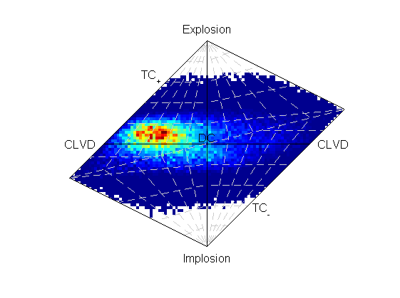
Hudson plot of the example results from examples/p_polarity.py (Plotted using MTplot MATLAB code)
Increasing the number of samples can improve the fit at the expense of time taken to run the inversion. Re-running the inversion with more samples (10,000,000) takes longer, but produces a better density of sampling (output file is P_Polarity_Example_Dense_OutputMT.mat).
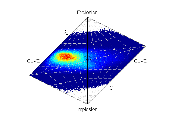
Hudson plot of the example results from examples/p_polarity.py (Plotted using MTplot MATLAB code)
4.3. P/SH Amplitude Ratio Inversion
Example script for running P/SH amplitude ratio inversion is examples/p_sh_amplitude_ratio.py
To run the script:
$ python p_sh_amplitude_ratio.py
The parameters used are:
- algorithm = 'iterate' - uses an iterative random sampling approach (see Random Monte Carlo sampling).
- parallel = True - tries to run in parallel using
multiprocessing.- phy_mem = 1 - uses a soft limit of 1Gb of RAM for estimating the sample sizes (This is only a soft limit, so no errors are thrown if the memory usage increases above this).
- dc = False - runs the full moment tensor inversion.
- max_samples = 1000000 - runs the inversion for 1,000,000 samples.
The Inversion object is created and then the forward model run with the results automatically outputted:
# Create the inversion object with the set parameters..
inversion_object = Inversion(data, algorithm=algorithm, parallel=parallel,
                             phy_mem=phy_mem, dc=dc, max_samples=max_samples,
                             convert=True)

# Run the forward model based inversion
inversion_object.forward()
The output file is P_SH_Amplitude_Ratio_Example_OutputMT.mat.
It is also possible to run the inversion for as many samples as possible in a given time (output file is P_Polarity_Example_Time_OutputMT.mat) by setting the parameters:
- algorithm = 'time' - uses an iterative random sampling approach (see Random Monte Carlo sampling) until a specified time has elapsed.
- max_time = 300 - runs the inversion for 300 seconds.
The Inversion object is created and then the forward model run with the results automatically outputted:
ns the inversion for a given time period.
rithm = 'time'
est:
# Run inversion for test
max_time = 10
:
# Length of time to run for in seconds.
max_time = 300
eate the inversion object with the set parameters..
rsion_object = Inversion(data, algorithm=algorithm, parallel=parallel,
                         phy_mem=phy_mem, dc=dc, max_time=max_time, convert=True)
n the forward model based inversion
rsion_object.forward()
4.4. Double-Couple Inversion
Sometimes it may be better to constrain the solution to only the double-couple space, this is easy to do from the command line using the -c flag (see MTfit command line options):
$ MTfit -c ...
An example script for running a mixed inversion constrained to double-couple space is examples/double_couple.py.
To run the script:
$ python double_couple.py
The inversion is run from a data file, which is the pickled (pickle/cPickle) data dictionary:
import cPickle
cPickle.dump(data, open('Double_Couple_Example.inv', 'wb'))
The inversion parameters used are:
- algorithm = 'iterate' - uses an iterative random sampling approach (see Random Monte Carlo sampling)
- parallel = True - tries to run in parallel using
multiprocessing- phy_mem = 1 - uses a soft limit of 1Gb of RAM for estimating the sample sizes (This is only a soft limit, so no errors are thrown if the memory usage increases above this)
- dc = True - runs the inversion in the double-couple space.
- max_samples = 100000 - runs the inversion for 100,000 samples.
Since the double-couple space has fewer dimensions than the moment tensor space, fewer samples are required for good coverage of the space, so only 100,000 samples are used.
The Inversion object is created and then the forward model run with the results automatically outputted:
# Create the inversion object with the set parameters.
inversion_object = Inversion(data_file='Double_Couple_Example.inv',
                             algorithm=algorithm, parallel=parallel,
                             phy_mem=phy_mem, dc=dc,
                             max_samples=max_samples, convert=True)
# Run the forward model based inversion
inversion_object.forward()
4.5. Time Limited Inversion
A different algorithm for the inverson can be set using the algorithm option. In this case the time constrained algorithm is used (for other options see MTfit.algorithms: Search Algorithms). An example script for running a time constrained inversion is examples/time_inversion.py.
To run the script:
$ python time_inversion.py
The time option for the inversion algorithm sets a maximum time (in seconds) to run the inversion for rather than a maximum number of samples. To select the algorithm from the command line use:
$MTfit --algorithm=time ...
For the other options see Command Line Options. The inversion parameters used in examples/time_inversion.py are:
- algorithm = 'time' - uses an time limited random sampling approach (see Random Monte Carlo sampling)
- parallel = False - runs in a single thread.
- phy_mem = 1 - uses a soft limit of 1Gb of RAM for estimating the sample sizes (This is only a soft limit, so no errors are thrown if the memory usage increases above this)
- dc = False - runs the inversion in the double-couple space.
- max_time = 120 - runs the inversion for 120 seconds.
- inversion_options = 'PPolarity,P/SHAmplitudeRatio' - Just uses PPolarity and P/SH Amplitude Ratios rather than all the data in the dictionary
In this case the inversion_options keyword argument is used to set the data types used in the inversion. If this is not set the inversion will use all of the available data types in the dictionary that match possible data types (see Inversion documentation), this is because the example data has other data types that are not desired or not independent:
>>> data.keys()=['PPolarity','P/SHRMSAmplitudeRatio','P/SVRMSAmplitudeRatio','P/SHAmplitudeRatio','UID]
The P/SHRMSAmplitudeRatio and the P/SHAmplitudeRatio are not independent, and so cannot both be used in this inversion.
The Inversion object is created and then the forward model run with the results automatically outputted:
# Create the inversion object with the set parameters.
inversion_object = Inversion(data, algorithm=algorithm, parallel=parallel,
                             phy_mem=phy_mem, dc=dc, inversion_options=inversion_options,
                             max_time=max_time, convert=True)

# Run the forward model based inversion
inversion_object.forward()
The output file is Time_Inversion_Example_OutputMT.mat.
It is also possible to run the inversion for the double-couple constrained inversion (output file is Time_Inversion_Example_OutputDC.mat):
dc = True
# Create the inversion object with the set parameters.
inversion_object = Inversion(data, algorithm=algorithm, parallel=parallel,
                             phy_mem=phy_mem, dc=dc, inversion_options=inversion_options,
                             max_time=max_time, convert=True)
# Run the forward model based inversion
inversion_object.forward()
4.6. Parallel MPI Inversion
Running the inversion using MPI on a multi-node environment (such as a cluster) is done from the command line using:
$ MTfit -M ...
Warning
Do not use the --mpi-call flag as this is a flag set automatically by the code
The script examples/mpi.py is an example script for running using MPI (It will test if mpi4py is installed)
The data file is pickled using cPickle:
# pickle data using cPickle
try:
    import cPickle as pickle
except ImportError:
    import pickle
# data saved to MPI_Example.inv using cPickle
with open('MPI_Example.inv', 'wb') as f:
    pickle.dump(f, data)
And then subprocess is used to call the inversion:
# Use subprocess to call MTfit
import subprocess
subprocess.call(['MTfit', '-M', '--data_file=MPI_Example.inv',
                 '--algorithm=iterate', '--max_samples=100000'])
This is equivalent to (see command line options for more information on the command line options):
$ MTfit -M --data_file=MPI_Example.inv --algorithm=iterate --max_samples=100000
The output file is MPI_Inversion_Example_OutputMT.mat.
The main advantage of running using MPI is to allow for more samples to be tried in a given time by using more processors.
4.7. Submitting to a Cluster
Submitting an MTfit job to a cluster using qsub uses a simple module called pyqsub (from https://www.github.com/djpugh/pyqsub) which provides command line options for running qsub.
To submit to the cluster from command line, on a computer with qsub available use:
$ MTfit -q ...
There are other available options when submitting to the cluster:
$ MTfit -q  --walltime=48:00:00 --nodes=4 --ppn=4 --pmem=2 --emailoptions=ae
    --email=example@example.com --name=MTfitClusterTest --queue=auto ...
This submits an MTfit job to the cluster using qsub (-q) with a walltime of 48 hours (--walltime) using 4 nodes (--nodes) and 4 processors per node (--ppn) with a maximum amount of physical memory per process of 2Gb (--pmem). The job will send emails on abort and end (--emailoptions) to email example@example.com (--email). It has a job name of MTfitClusterTest (--name) and is submitted to the auto queue (--queue).
These options, combined with the other command line options, will be saved to a job script named JobName.pJobID. For the above case, if the JobID was 207642 a PBS script is saved called
MTfitClusterTest.p207642
4.8. Inversion from a CSV File
MTfit can use a CSV file as input. An example CSV file can be made by running examples/make_csv_file.py in the examples folder:
$ python make_csv_file.py
This makes a CSV file (called csv_example_file.csv):
UID=Event1,,,,
PPolarity,,,,
Error,Name,TakeOffAngle,Measured,Azimuth
0.1,S0006,112.8,1,210.6
0.3,S0573,110.0,-1,306.7
0.1,S0563,131.4,-1,23.1
0.1,S0016,117.6,1,167.8
0.1,S0567,123.7,-1,41.3
0.1,S0654,110.0,-1,323.4
0.1,S0634,119.7,-1,342.5
0.1,S0533,138.3,-1,354.1
0.1,S0249,155.2,1,153.5
0.1,S0571,113.7,-1,54.5
0.1,S0065,125.6,1,184.2
0.1,S0095,127.4,1,159.2
0.1,S0537,134.9,-1,25.6
0.1,S0372,145.9,1,288.2
0.1,S0097,124.5,1,150.0
P/SHAmplitudeRatio,,,,
TakeOffAngle,Measured,Error,Name,Azimuth
112.8,1.91468406e-08   3.22758296e-08,9.58863666e-10   7.70965062e-09,S0006,210.6
110.0,4.88113677e-09   1.96675583e-08,2.45607268e-10   3.45469389e-09,S0573,306.7
131.4,1.45833761e-07   1.79089155e-09,7.28757867e-09   3.45820500e-09,S0563,23.1
117.6,9.31790661e-08   2.93385249e-08,4.65480572e-09   8.95408759e-09,S0016,167.8
123.7,1.20612039e-07   3.84818185e-08,6.02547046e-09   9.23059636e-09,S0567,41.3
110.0,2.07444768e-08   3.27506473e-08,1.03738569e-09   3.93335483e-09,S0654,323.4
119.7,7.83955802e-08   5.52997744e-08,3.91683797e-09   7.86172468e-10,S0634,342.5
138.3,1.38297893e-07   4.90243560e-08,6.91029070e-09   9.79988215e-10,S0533,354.1
155.2,1.74815653e-07   3.48061608e-08,8.75143170e-09   7.61184113e-10,S0249,153.5
113.7,8.41802958e-08   4.60234127e-08,4.20431936e-09   1.17189815e-08,S0571,54.5
125.6,1.09705743e-07   4.42081432e-08,5.48271153e-09   9.58851515e-10,S0065,184.2
127.4,1.35994091e-07   1.03528610e-08,6.79566727e-09   2.75097217e-09,S0095,159.2
134.9,1.54309735e-07   1.22170773e-08,7.71089395e-09   2.61801853e-09,S0537,25.6
145.9,6.88684554e-09   8.43199415e-08,3.43601244e-10   1.79928175e-09,S0372,288.2
124.5,1.24505851e-07   6.84587855e-09,6.22146156e-09   2.83710916e-09,S0097,150.0
,,,,
P/SVAmplitudeRatio,,,,
Name,Azimuth,Measured,Error,TakeOffAngle
S0006,210.6,3.22758296e-08   8.19892140e-08,7.70965062e-09   9.80424095e-09,112.8
S0573,306.7,1.96675583e-08   3.68506966e-08,3.45469389e-09   3.35913629e-09,110.0
S0563,23.1,1.79089155e-09   3.56992402e-08,3.45820500e-09   3.64333023e-09,131.4
S0016,167.8,2.93385249e-08   6.26397384e-08,8.95408759e-09   8.69575530e-09,117.6
S0567,41.3,3.84818185e-08   1.55744928e-08,9.23059636e-09   4.07140152e-09,123.7
S0654,323.4,3.27506473e-08   4.94388184e-08,3.93335483e-09   4.17167829e-09,110.0
S0634,342.5,5.52997744e-08   3.26269606e-08,7.86172468e-10   1.20208387e-09,119.7
S0533,354.1,4.90243560e-08   4.51596183e-08,9.79988215e-10   1.97681026e-09,138.3
S0249,153.5,3.48061608e-08   8.71989457e-08,7.61184113e-10   1.37314781e-09,155.2
S0571,54.5,4.60234127e-08   4.20042749e-09,1.17189815e-08   4.50190885e-09,113.7
S0065,184.2,4.42081432e-08   6.15020436e-08,9.58851515e-10   3.53524312e-09,125.6
S0095,159.2,1.03528610e-08   3.56854812e-08,2.75097217e-09   2.22496836e-09,127.4
S0537,25.6,1.22170773e-08   5.41945269e-08,2.61801853e-09   2.74678803e-09,134.9
S0372,288.2,8.43199415e-08   1.80916924e-08,1.79928175e-09   2.95196095e-10,145.9
S0097,150.0,6.84587855e-09   3.48806733e-08,2.83710916e-09   1.82493870e-09,124.5
,,,,
This is a CSV file with 2 events, one event ID of Event 1 with PPolarity and P/SHAmplitudeRatio and P/SVAmplitudeRatio data at 15 receivers, and a second event with no ID (will default to the event number, in this case 2) with PPolarity data at 15 receivers.
Running an inversion using a CSV file is the same as running a normal inversion. Calling from the command line is simply called by:
$ MTfit --datafile=thecsvfile.csv ...
The --invext flag sets the file ending that the inversion searches for when no datafile is specified, so to search for CSV files in the current directory:
$ MTfit --invext=csv
This will try to invert the data from all the CSV files in the current directory.
MTfit can be extended for other inversion file formats using setuptools entry-points
4.9. Location Uncertainty
MTfit can include location uncertainty in the resultant PDF. This requires samples from the location PDF. The location uncertainty is included in the inversion using a Monte Carlo method (see Bayesian Approach).
This file can be made from the NonLinLoc *.scat file using Scat2Angle in the pyNLLoc module.
The expected format for the location uncertainty file is:
Probability
StationName Azimuth TakeOffAngle
StationName Azimuth TakeOffAngle

Probability
.
.
.
e.g.:
504.7
S0271   231.1   154.7
S0649   42.9    109.7
S0484   21.2    145.4
S0263   256.4   122.7
S0142   197.4   137.6
S0244   229.7   148.1
S0415   75.6    122.8
S0065   187.5   126.1
S0362   85.3    128.2
S0450   307.5   137.7
S0534   355.8   138.2
S0641   14.7    120.2
S0155   123.5   117
S0162   231.8   127.5
S0650   45.9    108.2
S0195   193.8   147.3
S0517   53.7    124.2
S0004   218.4   109.8
S0588   12.9    128.6
S0377   325.5   165.3
S0618   29.4    120.5
S0347   278.9   149.5
S0529   326.1   131.7
S0083   223.7   118.2
S0595   42.6    117.8
S0236   253.6   118.6

502.7
S0271   233.1   152.7
S0649   45.9    101.7
S0484   25.2    141.4
S0263   258.4   120.7
.
.
.
MTfit can be extended to use other location PDF file formats using setuptools entry-points
Running with the location uncertainty included will slow the inversion as this requires more memory to store each of the location samples in the inversion. The number of samples used can be changed by setting the number_location_samples parameter in the Inversion object:
>>> import MTfit
>>> MTfit.Inversion(...,number_location_samples=10000,...)
This limits the number of station samples to 10,000, reducing the memory requirements and improving the speed.
The script examples/location_uncertainty.py contains an example for the location uncertainty inversion.
To run the script:
$ python location_uncertainty.py
The angle scatter file path option can be set from the command line using:
$ MTfit --anglescatterfilepath=./ --angleext=.scatangle ...
This will search in the current directory for scatangle files (default is to search for scatangle files if --angleext is not specified). The files are matched to the input data files if MTfit is called from the command line. A specific file or list of files can be set using:
$ MTfit --anglescatterfilepath=./thisanglefile.scatangle ...
Which uses the thisanglefile.scatangle file in the current directory.
The inversion parameters used in examples/location_uncertainty.py are:
- algorithm = 'time' - uses an time limited random sampling approach (see Random Monte Carlo sampling)
- parallel = True - runs in multiple threads using
multiprocessing.- phy_mem = 1 - uses a soft limit of 1Gb of RAM for estimating the sample sizes (This is only a soft limit, so no errors are thrown if the memory usage increases above this)
- dc = False - runs the inversion in the double-couple space.
- max_time = 60 - runs the inversion for 60 seconds.
- inversion_options = 'PPolarity' - Just uses PPolarity rather than all the data in the dictionary
- location_pdf_file_path = 'Location_Uncertainty.scatangle'
The Inversion object is created and then the forward model run with the results automatically outputted:
# Location uncertainty path
location_pdf_file_path = 'Location_Uncertainty.scatangle'
# Create the inversion object with the set parameters..
inversion_object = Inversion(data, location_pdf_file_path=location_pdf_file_path,
                             algorithm=algorithm, parallel=parallel, phy_mem=phy_mem, dc=dc,
                             inversion_options=inversion_options, max_time=max_time,
                             convert=True)
# Run the forward model based inversion
inversion_object.forward()
The output file is Location_Uncertainty_Example_OutputMT.mat.
Including the location uncertainty in an inversion is slower, since fewer samples are used in a given time. Setting the number of station samples parameter to a smaller number can reduce this:
# Reduce the number of station samples to increase the
# number of moment tensor samples tried
number_station_samples = 10000
# Create the inversion object with the set parameters..
inversion_object = Inversion(data, location_pdf_file_path=location_pdf_file_path,
                             algorithm=algorithm, parallel=parallel, phy_mem=phy_mem, dc=dc,
                             inversion_options=inversion_options, max_time=max_time,
                             number_station_samples=number_station_samples, convert=True)
# Run the forward model based inversion
inversion_object.forward()
This tries more samples, however it has a worse sampling of the location PDF than before. Taking this to extremes, reducing the number_location_samples to 100 improves the number of samples tried but reduces the quality of the location uncertainty sampling.
The method of including location uncertainty can also be used to include velocity model uncertainty by drawing location samples from a range of models and combining (see scripts/model_sampling.py).
4.10. Running from the Command Line
MTfit is easy to run from the command line. The installation should install a script onto the path so that:
$ MTfit -h
Gives the command line options. If this does not work see Running MTfit to install the script.
There are many command line options available (see MTfit command line options) but the default settings are usually ok.
examples/command_line.sh (*nix) or examples/command_line.bat is an example script for running the inversion from the command line:
#!/usr/bin/sh
echo "Command line MTfit example script\n"
echo "Needs MTfit to have been installed to run.\n"
echo "Making data file - csv_example_file.csv\n"
python make_csv_file.py

echo "MTfit --version:\n"
#Output MTfit version
MTfit --version

echo "Running MTfit from command line:\n"
echo "MTfit --data_file=csv_example*.inv --algorithm=iterate \
        --max_samples=100000 -b  --inversionoptions=PPolarity"
#Run MTfit from the command line. Options are:
#   --data_file=csv_example*.inv - use the data files matching csv_example*.inv
#   --algorithm=iterate - use the iterative algorithm
#   --max_samples=100000 - run for 100,000 samples
#   -b - carry out the inversion for both the double couple constrained
#           and full moment tensor spaces
#   --inversionoptions=PPolarity - carry out the inversion using
#           PPolarity data only
#   --convert - convert the solution using MTconvert.

MTfit --data_file=csv_example*.csv --algorithm=iterate --max_samples=100000 \
     -b  --inversionoptions=PPolarity --convert
This uses the data from the CSV example file (see Inversion from a CSV File), prints the version of MTfit being used and then calls MTfit from the command line. The parameters used are:
- --data_file=csv_*.inv - use the data files matching csv_*.inv
- --algorithm=iterate - use the iterative algorithm
- --max_samples=100000 - run for 100,000 samples
- -b - carry out the inversion for both the double couple constrained and full moment tensor spaces
- --inversionoptions=PPolarity - carry out the inversion using PPolarity data only
- --convert - convert the solution using
MTfit.MTconvert.
4.11. Scatangle file binning
Often the scatangle files are large with many samples at similar station angles. The size of these files can be reduced by binning these samples into similar bins. This can be done either before running MTfit or as a pre-inversion step using the command line parameters:
- --bin-scatangle=True - run the scatangle binning before the inversion
- --bin-size=1.0 - set a bin size of 1.0 degrees.
This can be run in parallel, which can speed up the process, using the same command line arguments as before.
The new files are outputted with _bin_1.0 appended if the bin-size is 1.0, and are automatically used in the inversio