11. Plotting the Moment Tensor¶

MTfit has a plotting submodule that can be used to represent the source. There are several different plot types, shown below, and MTplot can be used both from the command line, and from within the python interpreter.

This section describes how to use the plotting tools and shows the different plot types:

Beachball

Fault plane

Riedesel-Jordan

Radiation

Lune

Hudson

These are plotted using matplotlib, using a class based system. The main plotting class is the MTplot class, which stores the figure and handles the plotting, and each axes plotted is shown using a plot class from MTfit.plot.plot_classes. The plotting methods are designed to enable easy plotting without much user input, but also allow more complex plots to be made. The examples section shows two examples of using the plotting submodule.

The source code is shown in MTfit.plot.plot_classes.

Warning

matplotlib does not plot 3d plots very well, as each object is converted to a 2d object and plotted, and given a constant zorder for the whole plot. Consequently, the bi-axes plot (Chapman and Leaney, 2011) is not included as an option, and other 3D plots may not always work correctly.

For the full plot_classes documentation, see Plotting classes.

11.1. Using MTplot from the command line¶

MTplot can be run from the command line. A script should have been installed onto the path during installation and should be callable as:

$ MTplot

However it may be necessary to install the script manually. This is platform dependent.

11.1.1. Script Installation¶

11.1.1.1. Linux¶

Add this python script to a directory on the $PATH environmental variable:

#!/usr/bin/env python
import MTfit
MTfit.plot.__run__()

and make sure it is executable.

11.1.1.2. Windows¶

Add the linux script (above) to the path or if using powershell edit the powershell profile (usually found in Documents/WindowsPowerShell/ - if not present use $PROFILE|Format-List -Force to locate it, it may be necessary to create the profile) and add:

function MTplot{
    $script={
        python -c "import MTfit;MTfit.plot.__run__()" $args
        }
    Invoke-Command -ScriptBlock $script -ArgumentList $args
    }

Windows Powershell does seem to have some errors with commandline arguments, if necessary these should be enclosed in quotation marks e.g. "-d=datafile.inv"

11.1.2. Command Line Options¶

There are several command line options available, these can be found by calling:

$ MTplot -h

The command line defaults can be set using the same defaults file as for MTfit (see Running MTfit).

11.2. Using MTplot from the Python interpreter¶

Although MTplot can be run from the command line, it is much more powerful to run it from within the python interpreter. To run MTplot from the python interpreter, create the MTplot object:

>>> from MTfit.plot import MTplot
>>> MTplot(MTs,plot_type='beachball',stations={},plot=True,*args,**kwargs)

See Making the MTplot class for more information on the MTplot object.

11.3. Input Data¶

MTfit.plot.__core__.read() can read the three default output formats (MATLAB, hyp and pickle) for MTfit results.

Additional parsers can be installed using the MTfit.plot_read entry point described in Extending MTfit.

11.4. MTplot Class¶

The MTplot class is used to handle plotting the moment tensors. The moment tensors are stored as an MTData class.

class MTfit.plot.plot_classes.MTplot(MTs, plot_type='beachball', stations={}, plot=True, label=False, save_file='', save_dpi=200, *args, **kwargs)[source]¶

MTplot class - handles plotting of the moment tensor using different plot_classes

This object acts as a handle round a matplotlib figure, handling the moment tensors and creating the plot classes for axes.

Initialises the MTplot object.

Multiple plots (subplots) are handled using the matplotlib GridSpec - to create multiple plots, use nested lists for the MTs, with the inner lists corresponding to each column and the outer each row, e.g.:

[[x,y=1,1;x,y=2,1],[x,y=1,2;x,y=2,2]]

The total number of columns is given by the max number of points in the nested list. Lists with fewer points will have the last plot stretched to cover the remaining columns. Setting None in the list will stretch the plot to it's left to cover the columns.

The args and kwargs, which are passed through to the plot_class object can also be nested in this way. Additionally, if the parameters are equal to the number of columns, or number of rows, the same values are used for each plot in the corresponding column or row. If the dimension of the multiplot is square, the parameters are assumed to correspond to the rows.

Args: MTs: Moment tensor samples for creating MTData object, such as a numpy array of MT 6 vectors (see MTData initialisation for different types, and MTplot docstring for handling multiple plots
Keyword Args: plot_type: str - plot type selection (Default is 'beachball') stations: dict - Dictionary of stations, containing keys: 'names','azimuth','takeoff_angle' and 'polarity' or an empty dict (default) plot: bool - flag to actually plot and show the figure label: bool - flag to show axis labels if multiple plots are being shown save_file: string - filename to save plot to (if set) save_dpi: int - output dpi for file save args: passed through to plot_class initialisation kwargs: passed through to plot_class initialisation

ax_labels(show=True)[source]¶: Set or update axis label to axis corners.

plot(*args, **kwargs)[source]¶

Plots the figure and shows it.

Calls the plot functions for each plot_class in the multiplot.

11.5. MTData Class¶

The MTData class is used for storing and converting the moment tensors for plotting.

class MTfit.plot.plot_classes.MTData(MTs, probability=[], c=False, **kwargs)[source]¶

MTData object manages the moment tensors.

Additionally it enables conversion between different parameterisations and calculation of several statistics.

This is used by all of the plot classes for handling the moment tensor, and is transparent to converting and accessing the moment tensors, as it behaves like a numpy array (e.g. indexing and properties like shape are given for the moment tensor).

The MTData object also stores the probability, and is used for calculating the orientation mean.

MTData initialisation

Parameters corresponding to the moment tensor samples can be set as kwargs. These parameters include:

T, N, P, E, u, v, tau, k, gamma, delta, kappa, h, sigma, strike1, dip1, rake1, strike2, dip2, rake2, N1, N2

Args

MTs: numpy array of moment tensor six vectors with shape (6,n).: Alternatively, the input can be a dictionary from the MTfit output.

Keyword Args

probability: list or numpy array of probabilities - should be: the same length as the number of moment tensors, or empty (Default is [])
**kwargs: Attributes that correspond to converted parameters: of the moment tensor, as described above

cluster_normals()[source]¶

Cluster the normals.

This is a very simplistic algorithm that clusters the normals by dividing them into two groups with the shortest distance between them.

N.B. This depends on the initial values given, so if the normals are not well clustered, or the initial normals chosen are outliers, the results will not be a good clustering.

Consequently, only use this approach for well clustered fault plane normals (in at least one normal direction). The more tightly clustered normals are set to clustered_N1.

Returns: numpy array, numpy array, numpy array, numpy array: tuple of numpy arrays, clustered_N1, clustered_N2, clustered_rake1,clustered_rake2

get_max_probability(single=False)[source]¶

Returns an MTData object containing the maximum probability solutions

Keyword Args: single: bool - flag to return only one moment tensor (the first maximum probability moment tensor)

Returns:	New MTData object with max probability MT samples.
Return type:	MTData

get_mean()[source]¶

Calculates the mean moment tensor and variance of the moment tensor samples

Returns:	tuple of numpy arrays for the mean moment tensor six vector and the moment tensor six vector covariance.
Return type:	numpy array,numpy array

get_mean_orientation()[source]¶

Get the mean orientation from the clustered normals and rake parameters using the more tightly clustered parameters.

This also calculates the variance of the rake distributions and covariance of the clustered normals (using the probability if it is set)

Returns: numpy array, numpy array, numpy array: tuple of the mean strike dip and rake of the fault planes.

get_unique_McMC()[source]¶

Gets the unique McMC samples, with the probability scaled by the number of samples

Returns: MTData: New MTData object with unique MT samples and probabilities corresponding to the moment tensor frequencies.

is_dc()[source]¶: Returns array of DC values

11.6. Beachball plot¶

The simplest plot is a beachball plot using the MTfit.plot.plot_classes._AmplitudePlot class.

Using the MTplot function, it can be made with the following commands:

>>> import MTfit
>>> import numpy as np
>>> MTfit.plot.MTplot(np.array([[1],[0],[-1],[0],[0],[0]]),'beachball',
        fault_plane=True)

This plots the equal area projection of the source (a double-couple).

Stations can be included as a dictionary, with the azimuths and takeoff angles in degrees, such as:

>>> stations={'names':['S01','S02','S03','S04'],
              'azimuth':np.array([120.,5.,250.,75.]),
              'takeoff_angle':np.array([30.,60.,45.,10.]),
              'polarity':np.array([1,0,1,-1])}
>>> MTfit.plot.MTplot(np.array([[1],[0],[-1],[0],[0],[0]]),'beachball',
            stations=stations,fault_plane=True)

If the polarity probabilities have been used in the inversion, the probabilities can be plotted on the receivers, by setting the stations polarity array as an array of the larger polarity probabilities, with negative polarity probabilities corresponding to polarities in the negative direction, e.g.:

>>> stations={'names':['S01','S02','S03','S04'],
              'azimuth':np.array([120.,5.,250.,75.]),
              'takeoff_angle':np.array([30.,60.,45.,10.]),
              'polarity':np.array([0.8,0.5,0.7,-0.9])}
>>> MTfit.plot.MTplot(np.array([[1],[0],[-1],[0],[0],[0]]),'beachball',
            stations=stations,fault_plane=True)

To tweak the plot further, the plot class can be used directly:

>>> import MTfit
>>> import numpy as np
>>> X=MTfit.plot.plot_classes._AmplitudePlot(False,False,
        np.array([[1],[0],[-1],[0],[0],[0]]),'beachball',
        stations=stations,fault_plane=True)
>>> X.plot()

The first two arguments correspond to the subplot_spec and matplotlib figure to be used - if these are False, then a new figure is created.

It uses the MTfit.plot.plot_classes._AmplitudePlot class:

class MTfit.plot.plot_classes._AmplitudePlot(subplot_spec, fig, MTs, stations={}, phase='P', *args, **kwargs)[source]¶

Amplitude plotting (beachball)

parameter single is set to True, as can only plot one source per axis

Args: subplot_spec: matplotlib subplot spec fig: matplotlib figure MTs: moment tensor samples (see MTData initialisation docstring for formats)
Keyword Args: phase: str - phase to plot (default='p') lower: bool - project lower hemisphere (ie. downward hemisphere) full_sphere: bool - plot the full sphere fault_plane: bool - plot the fault planes nodal_line: bool - plot the nodal lines stations: dict - station dict containing keys: 'names','azimuth','takeoff_angle' and 'polarity' station_distribution: list - list of station dictionaries corresponding to a location PDF distribution show_zero_polarity: bool - flag to show zero polarity receivers show_stations: bool - flag to show stations when station_distribution present station_markersize: float - station marker size (squared to get area) station_colors: tuple - tuple of colors for negative, no, and positive polarity TNP: bool - show the TNP axes on the plot colormap: str - matplotlib colormap selection (using matplotlib.cm.get_cmap()) fontsize: int - fontsize for text linewidth: float - base linewidth (sometimes thinner or thicker values are used, but relative to this parameter) text: bool - flag to show or hide text on the plot axis_lines: bool - flag to show or hide axis lines on the plot resolution: int - resolution for spherical sampling etc

plot(MTs=False, *args, **kwargs)¶

Plots the result

Keyword Args: MTs: Moment tensors to plot (see MTData initialisation docstring for formats) args: args passed to the _ax_plot function (e.g. set local parameters to be different from initialisation values) kwargs: kwargs passed to the _ax_plot function (e.g. set local parameters to be different from initialisation values)

11.7. Fault Plane plot¶

A similar plot to the amplitude beachball plot is the fault plane plot, made using the MTfit.plot.plot_classes._FaultPlanePlot class.

Using the MTplot function, it can be made with the following commands:

>>> import MTfit
>>> import numpy as np
>>> MTfit.plot.MTplot(np.array([[1],[0],[-1],[0],[0],[0]]),'faultplane',
        fault_plane=True)

This plots the equal area projection of the source (a double-couple).

Stations can be included as a dictionary, like with the beachball plot.

The fault plane plot also can plot the solutions for multiple moment tensors, so the input array can be longer:

>>> import MTfit
>>> import numpy as np
>>> MTfit.plot.MTplot(np.array([[ 1,0.9, 1.1,0.4],
                                [ 0,0.1,-0.1,0.6],
                                [-1, -1,  -1, -1],
                                [ 0,  0,   0,  0],
                                [ 0,  0,   0,  0],
                                [ 0,  0,   0,  0]]),
                     'faultplane',fault_plane=True)

There are additional initialisation arguments, such as show_max_likelihood and show_mean boolean flags, which shows the maximum likelihood fault planes in the color given by the default color argument, and the mean orientation in green.

Additionally, if the probability argument is set, the fault planes are coloured by the probability, with more likely planes darker.

It uses the MTfit.plot.plot_classes._FaultPlanePlot class:

class MTfit.plot.plot_classes._FaultPlanePlot(subplot_spec, fig, MTs, stations={}, probability=[], phase='p', *args, **kwargs)[source]¶

Plots the fault plane distribution

parameter single is set to False as multiple sources can be plotted per axes

Args: subplot_spec: matplotlib subplot spec fig: matplotlib figure MTs: moment tensor samples (see MTData initialisation docstring for formats)
Keyword Args: probability: numpy array - moment tensor probabilities phase: str - phase to plot (default='p') lower: bool - project lower hemisphere (ie. downward hemisphere) full_sphere: bool - plot the full sphere fault_plane: bool - plot the fault planes nodal_line: bool - plot the nodal lines stations: dict - station dict containing keys: 'names','azimuth','takeoff_angle' and 'polarity' station_distribution: list - list of station dictionaries corresponding to a location PDF distribution show_zero_polarity: bool - flag to show zero polarity receivers show_stations: bool - flag to show stations when station_distribution present station_markersize: float - station marker size (squared to get area) station_colors: tuple - tuple of colors for negative, no, and positive polarity TNP: bool - show the TNP axes on the plot colormap: str - matplotlib colormap selection (using matplotlib.cm.get_cmap()) fontsize: int - fontsize for text linewidth: float - base linewidth (sometimes thinner or thicker values are used, but relative to this parameter) text: bool - flag to show or hide text on the plot axis_lines: bool - flag to show or hide axis lines on the plot resolution: int - resolution for spherical sampling etc show_max_likelihood: bool - show the maximum likelihood solution in the default color show_mean: bool - show the mean orientation source in green (thicker plane is better constrained) color: set color for maximum likelihood fault plane (show_max_likelihood)

plot(MTs=False, *args, **kwargs)¶

Plots the result

Keyword Args: MTs: Moment tensors to plot (see MTData initialisation docstring for formats) args: args passed to the _ax_plot function (e.g. set local parameters to be different from initialisation values) kwargs: kwargs passed to the _ax_plot function (e.g. set local parameters to be different from initialisation values)

11.8. Riedesel-Jordan plot¶

The Riedesel-Jordan plot is more complicated, and is described in Riedesel and Jordan (1989). It plots the source type on the focal sphere, in a region described by the source eigenvectors.

Using the MTplot function, it can be made with the following commands:

>>> import MTfit
>>> import numpy as np
>>> MTfit.plot.MTplot(np.array([[1],[0],[-1],[0],[0],[0]]),'riedeseljordan')

This plots the equal area projection of the source (a double-couple).

Stations cannot be shown on this plot.

The Riedesel-Jordan plot cannot plot the solutions for multiple moment tensors, so the input array can only be one moment tensor.

It uses the MTfit.plot.plot_classes._RiedeselJordanPlot class:

class MTfit.plot.plot_classes._RiedeselJordanPlot(subplot_spec, fig, MTs, *args, **kwargs)[source]¶

Plots the source as a Riedesel-Jordan type plot

Args: subplot_spec: matplotlib subplot spec fig: matplotlib figure MTs: moment tensor samples (see MTData initialisation docstring for formats)
Keyword Args: phase: str - phase to plot (default='p') lower: bool - project lower hemisphere (ie. downward hemisphere) full_sphere: bool - plot the full sphere fault_plane: bool - plot the fault planes nodal_line: bool - plot the nodal lines show_stations: bool - flag to show stations when station_distribution present station_markersize: float - sets the source type marker sizes (squared to get area) station_colors: tuple - tuple of colors for negative, no, and positive polarity TNP: bool - show the TNP axes on the plot colormap: str - matplotlib colormap selection (using matplotlib.cm.get_cmap()) color: str - matplotlib color for source region fontsize: int - fontsize for text linewidth: float - base linewidth (sometimes thinner or thicker values are used, but relative to this parameter) text: bool - flag to show or hide text on the plot axis_lines: bool - flag to show or hide axis lines on the plot resolution: int - resolution for spherical sampling etc

plot(MTs=False, *args, **kwargs)¶

Plots the result

Keyword Args: MTs: Moment tensors to plot (see MTData initialisation docstring for formats) args: args passed to the _ax_plot function (e.g. set local parameters to be different from initialisation values) kwargs: kwargs passed to the _ax_plot function (e.g. set local parameters to be different from initialisation values)

11.9. Radiation plot¶

The radiation plot shows the same pattern as the beachball plot, except the shape is scaled by the amplitude on the focal sphere.

Using the MTplot function, it can be made with the following commands:

>>> import MTfit
>>> import numpy as np
>>> MTfit.plot.MTplot(np.array([[1],[0],[-1],[0],[0],[0]]),'radiation')

This plots the equal area projection of the source (a double-couple).

Stations cannot be shown on this plot.

The radiation plot cannot plot the solutions for multiple moment tensors, so the input array can only be one moment tensor.

It uses the MTfit.plot.plot_classes._RadiationPlot class:

class MTfit.plot.plot_classes._RadiationPlot(subplot_spec, fig, MTs, stations={}, phase='P', *args, **kwargs)[source]¶

Plot the radiation pattern

Args: subplot_spec: matplotlib subplot spec fig: matplotlib figure MTs: moment tensor samples (see MTData initialisation docstring for formats)
Keyword Args: phase: str - phase to plot (default='p') lower: bool - project lower hemisphere (ie. downward hemisphere) full_sphere: bool - plot the full sphere fault_plane: bool - plot the fault planes nodal_line: bool - plot the nodal lines stations: dict - station dict containing keys: 'names','azimuth','takeoff_angle' and 'polarity' station_distribution: list - list of station dictionaries corresponding to a location PDF distribution show_zero_polarity: bool - flag to show zero polarity receivers show_stations: bool - flag to show stations when station_distribution present station_markersize: float - station marker size (squared to get area) station_colors: tuple - tuple of colors for negative, no, and positive polarity TNP: bool - show the TNP axes on the plot colormap: str - matplotlib colormap selection (using matplotlib.cm.get_cmap()) fontsize: int - fontsize for text linewidth: float - base linewidth (sometimes thinner or thicker values are used, but relative to this parameter) text: bool - flag to show or hide text on the plot axis_lines: bool - flag to show or hide axis lines on the plot resolution: int - resolution for spherical sampling etc

plot(MTs=False, *args, **kwargs)¶

Plots the result

Keyword Args: MTs: Moment tensors to plot (see MTData initialisation docstring for formats) args: args passed to the _ax_plot function (e.g. set local parameters to be different from initialisation values) kwargs: kwargs passed to the _ax_plot function (e.g. set local parameters to be different from initialisation values)

11.10. Hudson plot¶

The Hudson plot is a source type plot, described in Hudson et al. (1989). It plots the source type in a quadrilateral, depending on the chosen projection. There are two projections, the tau-k plot and the u-v plot, with the latter being more common (and the default).

Using the MTplot function, it can be made with the following commands:

>>> import MTfit
>>> import numpy as np
>>> MTfit.plot.MTplot(np.array([[1],[0],[-1],[0],[0],[0]]),'hudson')

This plots the u-v plot of the source (a double-couple).

Stations cannot be shown on this plot.

The Hudson plot can plot the solutions for multiple moment tensors, so the input array can be longer. Additionally, it can also plot a histogram of the PDF, if the probability argument is set.

It uses the MTfit.plot.plot_classes._HudsonPlot class:

class MTfit.plot.plot_classes._HudsonPlot(subplot_spec, fig, MTs, projection='uv', probability=[], **kwargs)[source]¶

Hudson plot class

Plots the source on the u-v or tau-k Hudson plot

Args: subplot_spec: matplotlib subplot spec fig: matplotlib figure MTs: moment tensor samples (see MTData initialisation docstring for formats)
Keyword Args: projection: str - select the projection type from uv or tauk [default is uv] probability: numpy array - moment tensor probabilities colormap: str - matplotlib colormap selection (using matplotlib.cm.get_cmap()) fontsize: int - fontsize for text linewidth: float - base linewidth (sometimes thinner or thicker values are used, but relative to this parameter) text: bool - flag to show or hide text on the plot axis_lines: bool - flag to show or hide axis lines on the plot resolution: int - resolution for spherical sampling etc grid_lines: bool - show the interior grid lines marginalised: bool - marginalise the PDF (defailt is True) color: set marker color type_label: bool - show the label of the different types hex_bin: bool - use the hex-bin histogram type (slightly smoother) bins: int/array/list of arrays - bins for numpy histogram call

plot(MTs=False, *args, **kwargs)¶

Plots the result

Keyword Args: MTs: Moment tensors to plot (see MTData initialisation docstring for formats) args: args passed to the _ax_plot function (e.g. set local parameters to be different from initialisation values) kwargs: kwargs passed to the _ax_plot function (e.g. set local parameters to be different from initialisation values)

11.11. Lune plot¶

The Lune plot is a source type plot, described in Tape and Tape (2012). It plots the source type in the fundamental eigenvalue lune, which can be projected into 2 dimensions.

Using the MTplot function, it can be made with the following commands:

>>> import MTfit
>>> import numpy as np
>>> MTfit.plot.MTplot(np.array([[1],[0],[-1],[0],[0],[0]]),'lune')

Stations cannot be shown on this plot.

The Lune plot can plot the solutions for multiple moment tensors, so the input array can be longer. Additionally, it can also plot a histogram of the PDF, if the probability argument is set.

It uses the MTfit.plot.plot_classes._LunePlot class:

class MTfit.plot.plot_classes._LunePlot(subplot_spec, fig, MTs, stations={}, phase='P', *args, **kwargs)[source]¶

Plots the source on the fundamental eigenvalue lune

Can be either a histogram or scatter plot.

parameter single is set to False as multiple sources can be plotted per axes

Args: subplot_spec: matplotlib subplot spec fig: matplotlib figure MTs: moment tensor samples (see MTData initialisation docstring for formats)
Keyword Args: phase: str - phase to plot (default='p') lower: bool - project lower hemisphere (ie. downward hemisphere) full_sphere: bool - plot the full sphere fault_plane: bool - plot the fault planes nodal_line: bool - plot the nodal lines stations: dict - station dict containing keys: 'names','azimuth','takeoff_angle' and 'polarity' station_distribution: list - list of station dictionaries corresponding to a location PDF distribution show_zero_polarity: bool - flag to show zero polarity receivers show_stations: bool - flag to show stations when station_distribution present station_markersize: float - station marker size (squared to get area) station_colors: tuple - tuple of colors for negative, no, and positive polarity TNP: bool - show the TNP axes on the plot colormap: str - matplotlib colormap selection (using matplotlib.cm.get_cmap()) fontsize: int - fontsize for text linewidth: float - base linewidth (sometimes thinner or thicker values are used, but relative to this parameter) text: bool - flag to show or hide text on the plot axis_lines: bool - flag to show or hide axis lines on the plot resolution: int - resolution for spherical sampling etc

plot(MTs=False, *args, **kwargs)¶

Plots the result

Keyword Args: MTs: Moment tensors to plot (see MTData initialisation docstring for formats) args: args passed to the _ax_plot function (e.g. set local parameters to be different from initialisation values) kwargs: kwargs passed to the _ax_plot function (e.g. set local parameters to be different from initialisation values)

11.12. Examples¶

This section shows a pair of simple examples and their results.

The first example is to plot the data from Krafla P Polarity example:

import MTfit
import numpy as np
#Load Data
st_dist=MTfit.plot.read('krafla_event_ppolarityDCStationDistribution.mat',
    station_distribution=True)
DCs,DCstations=MTfit.plot.read('krafla_event_ppolarityDC.mat')
MTs,MTstations=MTfit.plot.read('krafla_event_ppolarityMT.mat')
#Plot
plot=MTfit.plot.MTplot([np.array([1,0,-1,0,0,0]),DCs,MTs],
    stations=[DCstations,DCstations,MTstations],
    station_distribution=[st_dist,False,False],
    plot_type=['faultplane','faultplane','hudson'],fault_plane=[False,True,False],
    show_mean=False,show_max=True,grid_lines=True,TNP=False,text=[False,False,True])

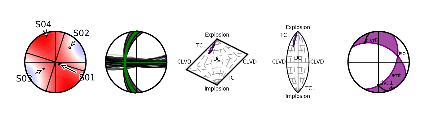
This produces a matplotlib figure:

Beachball plot showing the fault plane orientations for the double-couple constrained inversion and the marginalised source-type PDF for the full moment tensor inversion of the krafla data.

Beachball plots showing the station location uncertainty, and the fault plane orientations for the double-couple constrained inversion and the marginalised source-type PDF for the faultplane moment tensor inversion of the krafla data using polarity probabilities.

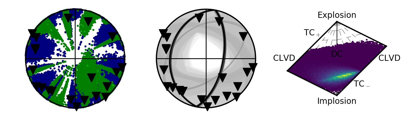
The second example shows the different plot types:

import MTfit
import numpy as np
import scipy.stats as sp
#Generate Data
n=100
DCs=MTfit.MTconvert.Tape_MT6(np.zeros(n),np.zeros(n),np.pi+0.1*np.random.randn(n),
        0.5+0.01*np.random.randn(n),0.1*np.random.randn(n))
probDCs=np.random.rand(n)
n=10000
g=-np.pi/12+0.01*np.random.randn(n)
d=np.pi/3+0.1*np.random.randn(n)
MTs=MTfit.MTconvert.Tape_MT6(g,d,np.pi+0.1*np.random.randn(n),
        0.5+0.01*np.random.randn(n),0.1*np.random.randn(n))
probMTs=sp.norm.pdf(g,-np.pi/12,0.01)*sp.norm.pdf(d,np.pi/3,0.1)
plot_sources=[np.array([1,0,1,-1,0,0]),DCs,MTs,MTs,np.array([1,0,1,-1,0,0])]
#Plot
plot=MTfit.plot.MTplot(plot_sources,
    plot_type=['beachball','faultplane','hudson','lune','riedeseljordan'],
    probability=[False,probDCs,probMTs,probMTs,False],
    colormap=['bwr','bwr','viridis','viridis','bwr'],
    stations=[{'names':['S01','S02','S03','S04'],
               'azimuth':np.array([120.,45.,238.,341.]),
               'takeoff_angle':np.array([12.,56.,37.,78.]),
               'polarity':[1,0,-1,-1]},{},{},{},{}],
    show_mean=True,show_max=True,grid_lines=True,TNP=False,fontsize=6,
    station_markersize=2,markersize=2)

This produces a matplotlib figure:

MTplot examples showing an equal area projection of a beachball for an example moment tensor source, fault plane distribution showing the mean orientation in green, Hudson and lune type plots of a full moment tensor PDF, and a Riedesel-Jordan type plot of an example moment tensor source.